Probability basics and set theory

The sample space $S$ of an experiment is the set of all possible outcomes of the experiment. An event $A$ is a subset of the sample space $S$, and we say that $A$ occurred if the actual outcome is in $A$.

De Morgan’s Laws

• $(A\cup B{)}^c=A^c\cap B^c$ , jo a or b me nhi hai vo a me bhi nhi hia aur b me bhi nhi hia

• $(A\cap B{)}^c=A^c\cup B^c$

Set theory notes

1. Intersection distributes over Union (just like numbers): $A\cap (B\cup C)=(A\cap B)\cup (A\cap C)$

2. Union distributes over Intersection (this is the one that breaks regular math logic): $A\cup (B\cap C)=(A\cup B)\cap (A\cup C)$

3. Commutative laws: $A\cup B=B\cup A$ and $A\cap B=B\cap A$

4. Associative laws: $(A\cup B)\cup C=A\cup (B\cup C)$ and $(A\cap B)\cap C=A\cap (B\cap C)$

5. Identity laws: $A\cup \varnothing =A$ and $A\cap S=A$

Naive definition of probability

Let $A$ be an event for an experiment with a finite sample space $S$.

The naive probability of $A$ is:

$P_{\text{naive}}(A)=\frac{|A|}{|S|}$

That is:

$P_{\text{naive}}(A)=\frac{\text{number of outcomes favorable to }A}{\text{total number of outcomes in }S}$

It's naive because it assumes outcomes to be equally likely, for example, heads and tails.

Counting

Multiplication rule

Consider a compound experiment consisting of two sub-experiments, Experiment A and Experiment B. Suppose that Experiment A has a possible outcome, and for each of those outcomes, Experiment B has b possible outcomes. Then the compound experiment has ab possible outcomes.

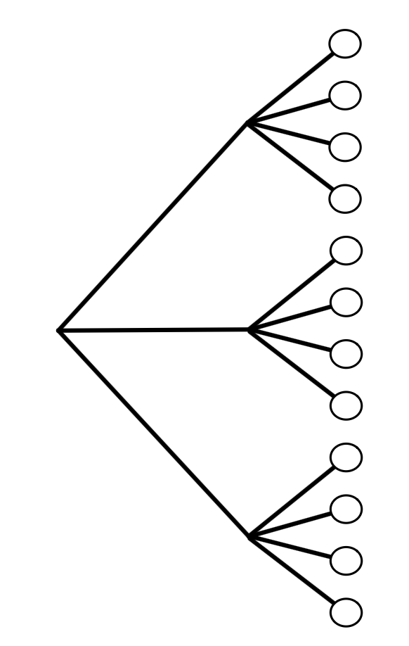
Q. Imagine you roll two standard 6-sided dice (a Red die and a Blue die) and you want to know how many different pairs of numbers you can get, where order doesn't matter (meaning a 3 and a 5 is the same thing as a 5 and a 3).

Ans. The trap is that you can’t just straight up divide by two. 36/2

---

Consider n objects and making k choices from them, one at a time with replacement

Then there are n^k possible outcomes

without replacement

N. N-1. N-2 …. N-k+1

Permutation of N objects -> N!

---

Birthday problem

(Birthday problem). There are k people in a room. Assume each

person’s birthday is equally likely to be any of the 365 days of the year (we exclude

February 29), and that people’s birthdays are independent (we will define indepen-

dence formally later, but intuitively it means that knowing some people’s birthdays

gives us no information about other people’s birthdays; this would not hold if, e.g.,

we knew that two of the people were twins). What is the probability that at least

one pair of people in the group have the same birthday?

Team problem

Example 1.4.13 (Committees and teams). Consider a group of four people.

(a) How many ways are there to choose a two-person committee?

(b) How many ways are there to break the people into two teams of two?

Binomial coefficient formula

For k ≤ n, we have

$$\left(\genfrac{}{}{0ex}{}{n}{k}\right)=\frac{n(n-1)\cdots (n-k+1)}{k!}=\frac{n!}{(n-k)!k!}.$$

For k > n, we have

$$\left(\genfrac{}{}{0ex}{}{n}{k}\right)=0.$$

Proof. Let $A$ be a set with $|A|=n$. Any subset of $A$ has size at most n, so $\left(\genfrac{}{}{0ex}{}{n}{k}\right)=0$ for k > n. Now let k ≤ n. By Theorem 1.4.8, there are $n(n-1)\cdots (n-k+1)$ ways to make an ordered choice of k elements without replacement. This overcounts each subset of interest by a factor of k!

I was not able to get a feel for why we divide by (k!), but then I thought about it like this. Suppose there are (x) ways to do an unordered selection of (k) elements from (n) elements. Once you have selected those (k) elements, there are (k!) ways to order them. You can think of these as two independent experiments, and because they are independent, their counts can be multiplied. Another way to see it is as branches of a tree: for every unordered selection, there are (k!) possible permutations. Therefore, the number of ordered selections is equal to the number of unordered selections multiplied by (k!). So if you know the number of ordered selections and want to find the number of unordered selections, you divide by (k!). In other words, the number of unordered selections equals the number of ordered selections divided by (k!).

Q. How many ways are there to permute the letters in the word STATISTICS?

Q. Which of the following events has the highest probability?

A: At least one 6 appears when 6 fair dice are rolled.

B: At least two 6’s appear when 12 fair dice are rolled.

Q. How many ways are there to choose k times from a set of n objects with replacement, if order doesn’t matter

don’t use this bose-einstien question above when events are not equi likely

As another example, with n= 365 days in a year and k people, how many possible unordered birthday lists are there? For example, for k = 3, we want to count lists like (May 1, March 31, April 11), where all permutations are considered equivalent. We can’t do a simple adjustment for overcounting such as nk/3! since, e.g., there are 6 permutations of (May 1, March 31, April 11) but only 3 permutations of (March 31, March 31, April 11). By Bose-Einstein, the number of lists isn+k−1 k . But the ordered birthday lists are equally likely, not the unordered lists, so the Bose-Einstein value should not be used in calculating birthday probabilities

Binomial identities

$$\left(\genfrac{}{}{0ex}{}{n}{k}\right)=\left(\genfrac{}{}{0ex}{}{n}{n-k}\right)$$$$n\left(\genfrac{}{}{0ex}{}{n-1}{k-1}\right)=k\left(\genfrac{}{}{0ex}{}{n}{k}\right)$$$$\left(\genfrac{}{}{0ex}{}{m+n}{k}\right)=\sum _{j=0}^k\left(\genfrac{}{}{0ex}{}{m}{j}\right)\left(\genfrac{}{}{0ex}{}{n}{k-j}\right)$$

Story proof : Consider a student organization consisting of mjuniors and nseniors, from which a committee of size k will be chosen. There are m+n k possibilities. If there are j juniors in the committee, then there must be k−j seniors in the committee. The right-hand side of the identity sums up the cases for j

$$\frac{(2n)!}{2^{n}n!}=(2n-1)(2n-3)\cdots 3\cdot 1$$

Q. The number of ways to break 2n people into n partnerships.
Ans. There are actually two ways to think about this.

---

Probability axioms

1. $P(\varnothing )=0$, $P(S)=1$.

2. If $A_1,A_2,\dots$ are disjoint events, then

$$P\left(\bigcup _{j=1}^{\infty }{A}_j\right)=\sum _{j=1}^{\infty }P(A_j).$$

Saying that these events are disjoint means that they are mutually exclusive: $A_i\cap A_j=\varnothing$ for $i\ne j$.

Any function $P$ (mapping events to numbers in the interval $[0,1]$ ) that satisfies the two axioms is considered a valid probability function. However, the axioms don’t tell us how probability should be interpreted; different schools of thought exist.

Frequentist and Bayesian interpretations

The frequentist view of probability is that it represents a long-run frequency over a large number of repetitions of an experiment: if we say a coin has probability $1/2$ of Heads, that means the coin would land Heads 50% of the time if we tossed it over and over and over.

The Bayesian view of probability is that it represents a degree of belief about the event in question, so we can assign probabilities to hypotheses like “candidate A will win the election” or “the defendant is guilty” even if it isn’t possible to repeat the same election or the same crime over and over again.

The Bayesian and frequentist perspectives are complementary, and both will be helpful for developing intuition in later chapters.

Some basic consequences of the axioms:

1. P(Aᶜ) = 1 - P(A).

2. If A ⊆ B, then P(A) ≤ P(B).

3. P(A ∪ B) = P(A) + P(B) - P(A ∩ B).

Inclusion-exclusion

For any events $A_1,\dots ,A_n$,

$$\begin{array}{rl}P\left(\bigcup _{i=1}^n{A}_i\right)& =\sum _{i}P(A_i)\\ & -\sum _{i<j}P(A_i\cap A_j)\\ & +\sum _{i<j<k}P(A_i\cap A_j\cap A_k)\\ & -\cdots \\ & +(-1{)}^{n+1}P(A_1\cap \cdots \cap A_n).\end{array}$$

Q. Consider a well-shuffled deck of n cards, labeled 1 through n. You flip over the cards one by one, saying the numbers 1 through n as you do so. You win the game if, at some point, the number you say aloud is the same as the number on the card being flipped over (for example, if the 7th card in the deck has the label 7). What is the probability of winning?

Ans. there are two ways to solve this question, one through inclusion exclusion and other through recursion.

Conditional probability

If A and B are events with P(B) > 0, then the conditional probability of A given B, denoted by $P(A|B)$, is defined as

$P(A|B)=\frac{P(A\cap B)}{P(B)}.$

Similarly, conditioning on both B and E means conditioning on their intersection:

$$P(A|B,E)=\frac{P(A\cap B\cap E)}{P(B\cap E)}.$$

From the definition of conditional probability,

$$P(A\cap B)=P(B)P(A|B)=P(A)P(B|A).$$

Probability of the intersection of n events

For any events A1, ..., An with P(A1 ∩ A2 ∩ ... ∩ A(n-1)) > 0,

$$P(A_1\cap A_2\cap \cdots \cap A_n)=P(A_1)P(A_2|A_1)P(A_3|A_1\cap A_2)\cdots P(A_n|A_1\cap \cdots \cap A_{n-1}).$$

The commas denote intersections, e.g. $P(A_3|A_1,A_2)$ is $P(A_3|A_1\cap A_2)$.

The intuition: drawing cards without replacement

Imagine you have a standard deck of 52 cards. You want to draw 3 cards from the top of the deck, one by one. You want to find the probability of a very specific outcome:

• $A_1$: Your 1st card is an Ace.

• $A_2$: Your 2nd card is a King.

• $A_3$: Your 3rd card is a Queen.

You want to find the probability that all three happen: $P(A_1\cap A_2\cap A_3)$. How do you calculate this naturally?

1. First, what is the probability that the 1st card is an Ace? There are 4 Aces out of 52 cards:

$$P(A_1)=\frac{4}{52}$$

1. Next, assuming you already drew that Ace, what is the probability that the 2nd card is a King? There are still 4 Kings left, but only 51 cards total remaining in the deck. This is a conditional probability:

$$P(A_2|A_1)=\frac{4}{51}$$

1. Finally, assuming you already have the Ace and the King out of the deck, what is the probability that the 3rd card is a Queen? There are 4 Queens left out of 50 cards remaining. This is:

$$P(A_3|A_1\cap A_2)=\frac{4}{50}$$

To find the final probability of the whole sequence, you just multiply them together:

$$P(A_1\cap A_2\cap A_3)=P(A_1)\times P(A_2|A_1)\times P(A_3|A_1\cap A_2)=\frac{4}{52}\times \frac{4}{51}\times \frac{4}{50}$$

Look at that! Your natural way of solving

note : if you look at the RHS of the formula it does not care about the order, but if you look at the LHS it would first look like it cares about the order but if you look closely it does not, because if it would have been than it would have written P(A2).P(A1/A2) as a saperate probbality and added that but they have’nt

Conditional versions of probability results

Any of the results we have derived about probability are still valid if we replace all unconditional probabilities with probabilities conditional on E. In particular:

• Conditional probabilities are between 0 and 1.

• P(S|E) = 1, P(∅|E) = 0.

• If A1, A2, ... are disjoint, then

$$P\left(\bigcup _{j=1}^{\infty }{A}_j\mid E\right)=\sum _{j=1}^{\infty }P(A_j|E).$$

• P(Aᶜ|E) = 1 - P(A|E).

• Inclusion-exclusion: P(A ∪ B|E) = P(A|E) + P(B|E) - P(A ∩ B|E).

Proof for the disjoint case. Define $\tilde{P}(A)=P(A|E)$. Second, if $A_1,A_2,\dots$ are disjoint events, then

P~(A1​∪A2​∪⋯)​=P(E)P​(A1​∩E)∪(A2​∩E)∪⋯​​​=P(E)∑j=1∞​P(Aj​∩E)​=j=1∑∞​P~(Aj​).​

LOTP with extra conditioning

Let $A_1,\dots ,A_n$ be a partition of $S$. Provided that P(Ai ∩ E) > 0 for all i, we have

$$P(B|E)=\sum _{i=1}^{n}P(B|A_i,E)P(A_i|E).$$

Law of total probability

Let $A_1,\dots ,A_n$ be a partition of the sample space $S$ (i.e., the $A_i$ are disjoint events and their union is $S$ ), with P(Ai) > 0 for all i. Then

$$P(B)=\sum _{i=1}^{n}P(B|A_i)P(A_i).$$

Proof. Since the $A_i$ form a partition of $S$, we can decompose $B$ as

$$B=(B\cap A_1)\cup (B\cap A_2)\cup \cdots \cup (B\cap A_n).$$

This is like chopping $B$ into the smaller pieces $B\cap A_1$ through $B\cap A_n$. By the second axiom of probability, because these pieces are disjoint, we can add their probabilities to get $P(B)$:

$$P(B)=P(B\cap A_1)+P(B\cap A_2)+\cdots +P(B\cap A_n).$$

Now we can apply the conditional probability multiplication rule to each of the $P(B\cap A_i)$:

$$P(B)=P(B|A_1)P(A_1)+\cdots +P(B|A_n)P(A_n).$$

Q. You have one fair coin, and one biased coin which lands Heads with probability 3/4. You pick one of the coins at random and flip it three times. It lands Heads all three times. Given this information, what is the probability that the coin you picked is the fair one?

Independence

Events A and B are independent if

$$P(A\cap B)=P(A)P(B).$$

If P(A) > 0 and P(B) > 0, then this is equivalent to

$$P(A|B)=P(A),$$

and also equivalent to $P(B|A)=P(B)$.

Independence is completely different from disjointness. If A and B are disjoint, then $P(A\cap B)=0$, so disjoint events can be independent only if P(A) = 0 or P(B) = 0. Knowing that A occurs tells us that B definitely did not occur, so A clearly conveys information about B, meaning the two events are not independent (except if A or B already has zero probability).

Consequences of event independence

If A and B are independent, then A and Bᶜ are independent, Aᶜ and B are independent, and Aᶜ and Bᶜ are independent.

Proof idea:

$$P(B^c|A)=1-P(B|A)=1-P(B)=P(B^c).$$

Independence of three events

Events A, B, and C are said to be independent if all of the following equations hold:

$$P(A\cap B)=P(A)P(B),$$$$P(A\cap C)=P(A)P(C),$$$$P(B\cap C)=P(B)P(C),$$$$P(A\cap B\cap C)=P(A)P(B)P(C).$$

If the first three conditions hold, we say that A, B, and C are pairwise independent.

Pairwise independence does not imply independence: it is possible that just learning about A or just learning about B is of no use in predicting whether C occurred, but learning that both A and B occurred could still be highly relevant for C.

On the other hand, $P(A\cap B\cap C)=P(A)P(B)P(C)$ does not imply pairwise independence; this can be seen quickly by looking at the extreme case P(A) = 0, when the equation becomes 0 = 0, which tells us nothing about B and C.

Independence of many events

For n events $A_1,A_2,\dots ,A_n$ to be independent, we require:

• Any pair to satisfy $P(A_i\cap A_j)=P(A_i)P(A_j)$ for i ≠ j.

• Any triplet to satisfy $P(A_i\cap A_j\cap A_k)=P(A_i)P(A_j)P(A_k)$ for i, j, k distinct.

• Similarly for all quadruplets, quintuplets, and so on.

This can quickly become unwieldy, but later we will discuss other ways to think about independence. For infinitely many events, we say that they are independent if every finite subset of the events is independent.

Conditional independence

Events A and B are said to be conditionally independent given E if

$$P(A\cap B|E)=P(A|E)P(B|E).$$

It is easy to make terrible blunders stemming from confusing independence and conditional independence.

• Two events can be conditionally independent given E, but not independent given Eᶜ.

• Two events can be conditionally independent given E, but not independent.

• Two events can be independent, but not conditionally independent given E.

In particular,

$$P(A\cap B)=P(A)P(B)$$

does not imply

$$P(A\cap B|E)=P(A|E)P(B|E).$$

Random variables

A random variable is a function from the sample space to the real numbers.

So if the sample space is S, then a random variable X takes one outcome from S as input and returns a real number for that outcome.

In notation:

$$X:S\to \mathbb{R}$$

The important thing is: a random variable is defined outcome by outcome. It looks at one outcome and assigns a number to it.

Example: tossing two coins

Suppose we toss two coins. The sample space is:

$$S=\{HH,HT,TH,TT\}$$

Now define a random variable X as the number of heads in the outcome.

Then:

• X(HH) = 2

• X(HT) = 1

• X(TH) = 1

• X(TT) = 0

So this random variable can take the values 0, 1, and 2.

The random variable could have been something else too. For example, another random variable could be whether the outcome has at least one head:

• X(HH) = 1

• X(HT) = 1

• X(TH) = 1

• X(TT) = 0

Here 1 means “yes, at least one head” and 0 means “no heads”.

Discrete and continuous random variables

Random variables can be discrete or continuous.

A discrete random variable takes countable values, like 0, 1, 2, 3, and so on.

A continuous random variable can take values over an interval, like any real number between 0 and 1.

One subtle point: even if the sample space is continuous, the random variable can still be discrete.

For example, suppose a person arrives at a bus stop at some random time between 0 and 60 minutes. The sample space is continuous because the arrival time could be 12.1 minutes, 12.11 minutes, 12.111 minutes, and so on.

But define X like this:

• X = 1 if the person arrives in the first 30 minutes

• X = 0 if the person arrives after 30 minutes

Here the sample space is continuous, but the random variable X is discrete because it only takes two values: 0 and 1.

What a random variable is allowed to look at

A random variable can only look at the outcome it is being applied to. It cannot look across all outcomes and calculate something global about the whole sample space.

For example, if we toss two coins, it is not correct to define a random variable as “the probability of getting at least one head”. That probability needs us to look across multiple outcomes in the sample space.

But it is completely fine to define a random variable as “does this outcome have at least one head?”

That random variable only looks at the single outcome:

• HH has at least one head, so X(HH) = 1

• HT has at least one head, so X(HT) = 1

• TH has at least one head, so X(TH) = 1

• TT has no head, so X(TT) = 0

So the difference is:

• Probability of at least one head: talks about the whole experiment/sample space.

• Indicator random variable for at least one head: talks about one outcome at a time and returns 1 or 0.

Probabilities of values of a random variable

Once we have assigned a random variable to the outcomes, we can use it to calculate probabilities over specific values of that random variable.

For example, suppose X is the number of heads in two coin tosses. Then we can ask questions like:

• What is P(X = 1)?

• What is P(X > 1)?

These are really questions about which outcomes in the sample space make the random variable take that value.

For two coin tosses:

• X = 1 happens for HT and TH, so P(X = 1) = P({HT, TH}).

• X > 1 happens only for HH, so P(X > 1) = P({HH}).

So after defining X, we stop talking directly about raw outcomes and start talking about events like X = 1, X > 1, X ≤ 2, and so on.

Probability mass function

For a discrete random variable, the probability mass function (PMF) tells us how much probability mass each possible value of the random variable gets.

Think of it like a graph:

• On the x-axis, write all the values the random variable can take.

• On the y-axis, write the probability that the random variable is equal to that value.

For example, if X is the number of heads in two fair coin tosses, then X can take the values 0, 1, and 2.

The PMF is:

xP(X = x)00.2510.5020.25

So the graph would put probability mass 0.25 on 0, probability mass 0.50 on 1, and probability mass 0.25 on 2.

The important thing is that all the probabilities in a PMF must add up to 1:

$$P(X=0)+P(X=1)+P(X=2)=1$$

In general:

$$\sum _{x}P(X=x)=1$$

So a PMF shows how the total probability mass is distributed across the possible values of a discrete random variable.

Bernoulli trial

An experiment that can result in either a “success” or a “failure” (but not both) is called a Bernoulli trial.

A Bernoulli random variable can be thought of as the indicator of success in a Bernoulli trial: it equals 1 if success occurs and 0 if failure occurs.

The important clarification: a Bernoulli trial does not mean the underlying sample space S must have only two outcomes. It means we are viewing the sample space through a binary lens, using a random variable that collapses the outcome into exactly two values:

• 1 for success

• 0 for failure

Case 1: the sample space is already binary

Experiment: flip a single coin.

$$S=\{H,T\}$$

Define X by:

• X(H) = 1

• X(T) = 0

Here, both the sample space and the random variable are naturally binary.

Case 2: the sample space has many outcomes, but the random variable is binary

Example: roll a die.

$$S=\{1,2,3,4,5,6\}$$

There are 6 outcomes. But define X as: “did I roll a 6?”

$$X(s)=\{\begin{array}{ll}1& \text{if }s=6\\ 0& \text{if }s\in \{1,2,3,4,5\}\end{array}$$

The underlying experiment has 6 outcomes, but X is still a Bernoulli random variable because it only takes the values 0 and 1.

Case 3: the sample space is continuous, but the random variable is binary

Suppose we measure the exact lifespan of a laptop battery in hours.

$$S=[0,\infty )$$

There are infinitely many possible outcomes. But define Y as: “does the battery last more than 5 hours?”

$$Y(s)=\{\begin{array}{ll}1& \text{if }s>5\\ 0& \text{if }s\le 5\end{array}$$

This is also a Bernoulli random variable. The sample space is continuous, but the random variable only outputs 0 or 1.

Binomial distribution

Suppose that n independent Bernoulli trials are performed, each with the same success probability p. Let X be the number of successes.

The distribution of X is called the Binomial distribution with parameters n and p.

We write $X\sim Bin(n,p)$ to mean that X has the Binomial distribution with parameters n and p, where n is a positive integer and 0 < p < 1.

Binomial PMF

If $X\sim Bin(n,p)$, then the PMF of X is

$$P(X=k)=\left(\genfrac{}{}{0ex}{}{n}{k}\right)p^k(1-p{)}^{n-k}.$$

You should be able to derive this yourself.

Theorem 3.3.7

Let $X\sim Bin(n,p)$, and let q = 1 - p. We often use q to denote the failure probability of a Bernoulli trial.

Then:

$$n-X\sim Bin(n,q).$$

Hypergeometric distribution

Consider an urn with w white balls and b black balls. We draw n balls out of the urn at random without replacement, such that all samples of size n from the w + b balls are equally likely.

Let X be the number of white balls in the sample. Then X is said to have the Hypergeometric distribution with parameters w, b, and n. We denote this by:

$$X\sim HGeom(w,b,n)$$

With replacement vs. without replacement

Imagine an urn with w = 6 white balls and b = 4 black balls. Total balls = 10. You want to draw n = 5 balls.

With replacement (Binomial): You draw a ball, write down its color, and put it back. Every single time you reach into the urn, the probability of getting a white ball is exactly the same:

$$\frac{w}{w+b}=\frac{6}{10}$$

Because the probability never changes, these are independent Bernoulli trials, which is exactly the setup for a Binomial distribution.

Without replacement (Hypergeometric): You draw a ball and keep it out. Now, the universe changes after every draw. If you draw a white ball first, there are fewer white balls left, so the probability of getting a white ball on the next turn drops.

Because the trials are dependent, the Binomial formula breaks. We need a new tool: the Hypergeometric distribution.

Breaking down the Hypergeometric PMF formula

The probability of getting exactly k white balls in your sample of size n is:

$$P(X=k)=\frac{\left(\genfrac{}{}{0ex}{}{w}{k}\right)\left(\genfrac{}{}{0ex}{}{b}{n-k}\right)}{\left(\genfrac{}{}{0ex}{}{w+b}{n}\right)}$$

Discrete uniform distribution

We write:

$$X\sim \text{DUnif}(C)$$

The core story

You choose exactly one number from a finite set of possibilities, where every single choice has the exact same likelihood of being picked. This is the random variable version of the naive definition of probability.

• Parameter: C is a finite, nonempty set of numbers (the choices).

• Size: |C| represents the total count of elements inside that set.

The probability mass function (PMF)

Because the total probability of all choices must sum to 1, the probability of picking any specific single number x is completely locked in by the size of the set:

$$p_X(x)=P(X=x)=\{\begin{array}{ll}\frac{1}{|C|}& \text{if }x\in C\\ 0& \text{otherwise}\end{array}$$

Calculating subsets (events)

If you want to find the probability that your chosen number falls into a specific target group A, where A is a subset of C, the problem simplifies to basic counting:

$$P(X\in A)=\frac{|A|}{|C|}=\frac{\text{Number of favorable options}}{\text{Total number of options}}$$

Key takeaways for intuition

• Uniform = perfectly equal: You cannot ch

Cumulative distribution function

Unlike the PMF, which only discrete random variables possess, the CDF is defined for all random variables.

Definition 3.6.1

The cumulative distribution function (CDF) of a random variable X is the function $F_X$ given by:

$$F_X(x)=P(X\le x)$$

The CDF of a discrete random variable consists of jumps and flat regions.

The height of a jump in the CDF at x is equal to the value of the PMF at x.

Valid CDFs

Any CDF F has the following properties.

1. Increasing: If x1 ≤ x2, then F(x1) ≤ F(x2).

2. Right-continuous: the CDF is continuous except possibly for having some jumps. Wherever there is a jump, the CDF is continuous from the right. That is, for any a, we have

$$F(a)=\underset{x\to a^{+}}{\lim }F(x)$$

1. Convergence to 0 and 1 in the limits:

$$\underset{x\to -\infty }{\lim }F(x)=0$$

and

$$\underset{x\to \infty }{\lim }F(x)=1$$

A concrete example: rolling a die

Let X be the result of a fair 6-sided die roll. Let’s look at the CDF at a = 3, which means finding:

$$F(3)=P(X\le 3)$$

Because a die can only land on whole numbers, the graph of this CDF looks like a staircase.

For any number just below 3, like 2.99, the probability $P(X\le 2.99)$ is only $2/6$, because you could have rolled a 1 or a 2.

The left side: ${\lim }_{x\to -\infty }F(x)=0$

What it says in plain English: as you move infinitely far to the left on the x-axis, the value of the CDF drops to exactly 0.

The intuition: remember that F(x) represents $P(X\le x)$.

Functions of random variables

A function of a random variable is also a random variable.

That is, if X is a random variable, then $X^2$, $e^X$, and $\sin (X)$ are also random variables, as is $g(X)$ for any function $g:\mathbb{R}\to \mathbb{R}$.

Suppose we define a new random variable:

$$Y=g(X)$$

How do we find the PMF of this new variable Y?

If we already know the PMF of X, then we find the probabilities of Y by looking at which values of X get mapped to each value of Y.

One-to-one case

If g is one-to-one, every unique input gives a unique output. There are no duplicates or ties.

Examples:

• $g(x)=2x$ is one-to-one.

• $g(x)=\sqrt{x}$ is one-to-one on nonnegative x.

• $g(x)=x^2$ is not one-to-one on all real numbers, because both 2 and -2 map to 4.

If g is one-to-one, the probabilities do not change. Only the labels change.

Concrete example

Let X have the following PMF:

• $P(X=1)=0.2$

• $P(X=2)=0.5$

• $P(X=3)=0.3$

Now define:

$$Y=10X$$

Here $g(x)=10x$, which is one-to-one.

The possible values of Y are 10, 20, and 30. The probabilities stay exactly the same:

• $P(Y=10)=P(X=1)=0.2$

• $P(Y=20)=P(X=2)=0.5$

• $P(Y=30)=P(X=3)=0.3$

PMF of g(X)

Let X be a discrete random variable and let $g:\mathbb{R}\to \mathbb{R}$.

The support of $g(X)$ is the set of all y such that $g(x)=y$ for at least one x in the support of X.

The PMF of $g(X)$ is:

$$P(g(X)=y)=\sum _{x:g(x)=y}P(X=x)$$

This is the rule when g is not one-to-one: collect all the x values that collapse into the same y value, and add their probabilities.

For example, if $Y=X^2$, then both X = 2 and X = -2 map to Y = 4. So:

$$P(Y=4)=P(X=2)+P(X=-2)$$

Functions of two random variables

Given an experiment with sample space S, if X and Y are random variables that map $s\in S$ to X(s) and Y(s) respectively, then $g(X,Y)$ is the random variable that maps s to $g(X(s),Y(s))$.

When you move from a function of one random variable, $g(X)$, to a function of two random variables, $g(X,Y)$, you are combining two inputs to create a single output.

Examples:

• $g(X,Y)=X+Y$

• $g(X,Y)=X\cdot Y$

• $g(X,Y)=\max (X,Y)$

From first principles, the one-to-one and many-to-one logic works the same way as before, but now the inputs are pairs $(x,y)$ instead of single values x.

The one-to-one case

For $g(X,Y)$ to be one-to-one, every unique pair of inputs $(x,y)$ must give a unique output.

If that happens, you just change the label and keep the probability of that specific pair:

$$P(g(X,Y)=z)=P(X=x,Y=y)$$

where z is the unique value produced by the pair $(x,y)$.

This is extremely rare for normal functions of two variables.

For example, addition is not one-to-one. The output 3 can come from many pairs:

• (1, 2)

• (2, 1)

• (0, 3)

• (4, -1)

An example of a one-to-one two-variable function can be something like:

$$g(X,Y)=10X+Y$$

if X and Y are single-digit integers.

If X = 2 and Y = 3, then g(2,3) = 23. No other pair of single digits gives 23, so:

$$P(g(X,Y)=23)=P(X=2,Y=3)$$

The many-to-one case

This is the standard case.

Functions like $X+Y$, $X-Y$, or $\max (X,Y)$ naturally collapse many distinct pairs $(x,y)$ into the same final value z.

So we use the same collapsing/summing rule as before, except now we sum over pairs:

$$P(g(X,Y)=z)=\sum _{(x,y):g(x,y)=z}P(X=x,Y=y)$$

When you take a function of two random variables, $g(X,Y)$, you are doing dimensional reduction: you are taking a two-dimensional grid of possibilities and flattening it down onto a single one-dimensional number line

Independence of two random variables

Random variables X and Y are said to be independent if, for all real numbers x and y,

$$P(X\le x,Y\le y)=P(X\le x)P(Y\le y).$$

In the discrete case, this is equivalent to:

$$P(X=x,Y=y)=P(X=x)P(Y=y).$$

Independence of many random variables

Random variables X1, ..., Xn are independent if, for all real numbers x1, ..., xn,

$$P(X_1\le x_1,...,X_n\le x_n)=P(X_1\le x_1)...P(X_n\le x_n).$$

For infinitely many random variables, we say that they are independent if every finite subset of the random variables is independent.

This looks simpler than independence for many events, where we had to check pairs, triplets, and so on. But here the equality has to hold for all possible values x1, ..., xn. That is infinitely many conditions. If we can find even one list of values where the equality fails, then the random variables are not independent.

Why group independence implies pairwise independence

For three random variables, independence says:

$$P(X_1\le x_1,X_2\le x_2,X_3\le x_3)=P(X_1\le x_1)P(X_2\le x_2)P(X_3\le x_3).$$

What if we only want to prove that X1 and X2 are independent, ignoring X3?

The trick is to push x3 all the way to infinity.

As x goes to ∞, a CDF becomes 1. So P(X3 ≤ ∞) becomes 1 and vanishes from both sides.

We are left with:

$$P(X_1\le x_1,X_2\le x_2)=P(X_1\le x_1)P(X_2\le x_2).$$

So if a whole group is independent, any pair you pick out of that group is also independent. This is pairwise independence.

Functions of independent random variables

If X and Y are independent random variables, then any function of X is independent of any function of Y.

Independent and identically distributed (i.i.d.)

We often work with random variables that are independent and have the same distribution. We call such random variables independent and identically distributed, or i.i.d. for short.

Independent vs. identically distributed

“Independent” and “identically distributed” are two often-confused but completely different concepts.

Random variables are independent if they provide no information about each other.

Random variables are identically distributed if they have the same PMF, or equivalently the same CDF.

Whether two random variables are independent has nothing to do with whether they have the same distribution.

Theorem 3.8.8

If X ∼ Bin(n,p), viewed as the number of successes in n independent Bernoulli trials with success probability p, then we can write:

$$X=X_1+...+X_n$$

where the Xi are i.i.d. Bern(p).

Theorem 3.8.9

If X ∼ Bin(n,p), Y ∼ Bin(m,p), and X is independent of Y, then:

$$X+Y\sim Bin(n+m,p).$$

For these two theorems, looking for a heavy mathematical proof is kind of stupid. You can just think through them logically and they make sense.

Conditional independence of random variables

Random variables X and Y are conditionally independent given a random variable Z if, for all real numbers x and y and all z in the support of Z,

$$P(X\le x,Y\le y|Z=z)=P(X\le x|Z=z)P(Y\le y|Z=z).$$

For discrete random variables, an equivalent definition is:

$$P(X=x,Y=y|Z=z)=P(X=x|Z=z)P(Y=y|Z=z).$$

This is the definition of independence, except that we condition on Z = z everywhere, and require the equality to hold for all z in the support of Z.

Conditional PMF

For any discrete random variables X and Z, the function P(X=x|Z=z), when considered as a function of x for fixed z, is called the conditional PMF of X given Z = z.

Fisher exact test

A scientist wishes to study whether women or men are more likely to have a certain disease, or whether they are equally likely.

A random sample of n women and m men is gathered, and each person is tested for the disease. Assume the test is completely accurate.

The numbers of women and men in the sample who have the disease are X and Y respectively, with X ∼ Bin(n,p1) and Y ∼ Bin(m,p2), independently.

Here p1 and p2 are unknown, and we are interested in testing whether p1 = p2. This is known as a null hypothesis in statistics.

Now suppose p1 = p2.

Suppose X + Y = r. Then find the conditional probability of X = x given X + Y = r.

By Bayes’ rule:

$$P(X=x|X+Y=r)=\frac{P(X+Y=r|X=x)P(X=x)}{P(X+Y=r)}$$

Since X + Y = r and X = x means Y = r - x,

$$P(X=x|X+Y=r)=\frac{P(Y=r-x)P(X=x)}{P(X+Y=r)}.$$

Theorem 3.9.2

If X ∼ Bin(n,p), Y ∼ Bin(m,p), and X is independent of Y, then the conditional distribution of X given X + Y = r is:

$$HGeom(n,m,r).$$

Theorem 3.9.3

If X ∼ HGeom(w,b,n) and N = w + b goes to ∞ such that

$$p=\frac{w}{w+b}$$

remains fixed, then the PMF of X converges to the Bin(n,p) PMF.

Why we cannot just let w or b go to infinity separately

If w and b move separately, the nature of the problem collapses.

Scenario A: b goes to infinity but w stays fixed. If there are only w = 5 white balls and the black balls grow to infinity, then the proportion of white balls becomes 0. If you draw n balls from this urn, you will get exactly 0 white balls every single time. It becomes deterministic and uninteresting.

Scenario B: w goes to infinity but b stays fixed. Then the proportion of white balls becomes 1. If you draw n balls, you will get n white balls every single time.

Expectation

For a discrete random variable $X$ with possible values $x_j$,

$$E(X)=\sum _j{x}_{j}P(X=x_j).$$

Let $X\sim Bern(p)$ and $q=1-p$. Then

$$E(X)=1p+0q=p.$$

Expectation depends only on distribution

If $X$ and $Y$ are discrete random variables with the same distribution, then

$$E(X)=E(Y)$$

if either side exists.

Linearity of expectation

For any random variables $X,Y$ and any constant $c$,

$$E(X+Y)=E(X)+E(Y),$$$$E(cX)=cE(X).$$

Binomial expectation

For $X\sim Bin(n,p)$, let’s find $E(X)$.

This is that you can write it as a sum of $n$ Bernoullis, right?

$$X=X_1+X_2+\cdots +X_n$$

where each $X_i\sim Bern(p)$.

And so you can take expectation on both sides using linearity of expectation:

$$E(X)=E(X_1)+E(X_2)+\cdots +E(X_n)$$

Since each Bernoulli has expectation $p$,

$$E(X)=p+p+\cdots +p=np.$$

Make sense?

Hypergeometric expectation

Let $X\sim HGeom(w,b,n)$, interpreted as the number of white balls in a sample of size $n$ drawn without replacement from an urn with $w$ white and $b$ black balls.

As in the Binomial case, we can write $X$ as a sum of Bernoulli random variables:

$$X=I_1+\cdots +I_n,$$

where $I_j$ equals 1 if the $j$ th ball in the sample is white and 0 otherwise.

By symmetry,

$$I_j\sim Bern(p)$$

with

$$p=\frac{w}{w+b},$$

since unconditionally the $j$ th ball drawn is equally likely to be any of the balls.

Unlike in the Binomial case, the $I_j$ are not independent, since the sampling is without replacement: given that a ball in the sample is white, there is a lower chance that another ball in the sample is white.

However, linearity still holds for dependent random variables. Thus,

$$E(X)=\frac{nw}{w+b}.$$

So, the first time when I read this, I was shocked because if you look at this, you can break it down as indicators: $I_1,I_2,\dots ,I_n$, where each one is asking whether that draw is a white ball.

Now they have taken the individual probabilities for the expectations and just added them.

The issue is that they are indicator random variables, so each one is 0 or 1, right?

Now, the issue is, you are saying that the probability changes after I pick the first ball. It does change conditionally. But unconditionally, the probability that the $j$ th ball is white is still

$$\frac{w}{w+b}.$$

Okay, makes sense.

But for calculating the probability of the whole sequence, dependence matters. There we cannot simply multiply individual probabilities like in the Binomial case. We would have to take the conditional probability route.

But for expectation, we are not multiplying the indicators. We are adding them. And linearity of expectation works even when the random variables are dependent.

Make sense?

Geometric distribution

Consider a sequence of independent Bernoulli trials, each with the same success probability $p\in (0,1)$, with trials performed until a success occurs.

Let $X$ be the number of failures before the first successful trial. Then $X$ has the Geometric distribution with parameter $p$ ; we denote this by

$$X\sim Geom(p).$$

If $q=1-p$, then

$$P(X=k)=q^{k}p$$

for $k=0,1,2,\dots$.

The expectation is

$$E(X)=\frac{q}{p}.$$

Geometric CDF

If $X\sim Geom(p)$, then the CDF of $X$ is

$$F(x)=\{\begin{array}{ll}1-q^{\lfloor x\rfloor +1}& \text{if }x\ge 0,\\ 0& \text{if }x<0.\end{array}$$

Negative Binomial distribution

In a sequence of independent Bernoulli trials with success probability $p$, if $X$ is the number of failures before the $r$ th success, then $X$ is said to have the Negative Binomial distribution with parameters $r$ and $p$, denoted

$$X\sim NBin(r,p).$$

Negative Binomial PMF

If $X\sim NBin(r,p)$, then the PMF of $X$ is

$$P(X=n)=\left(\genfrac{}{}{0ex}{}{n+r-1}{r-1}\right)p^r{q}^n$$

for $n=0,1,2,\dots$, where $q=1-p$.

Theorem 4.3.10

Let $X\sim NBin(r,p)$, viewed as the number of failures before the $r$ th success in a sequence of independent Bernoulli trials with success probability $p$.

Then we can write

$$X=X_1+\cdots +X_r$$

where the $X_i$ are i.i.d. $Geom(p)$.

A Negative Binomial random variable is just a collection of independent Geometric random variables stacked back-to-back.

Concrete timeline

Imagine you are tossing a coin where Heads = Success ( $S$ ) and Tails = Failure ( $F$ ). You want to keep tossing until you see a total of $r=3$ successes.

Let $X$ be the total number of failures you accumulate before that 3rd success happens. By definition,

$$X\sim NBin(3,p).$$

Suppose you start flipping, and this is the exact sequence of outcomes you get:

$$FFSFSFFFS$$

Let's divide this timeline into eras, using the successes as the borders:

• Era 1, before the 1st success: you flipped $F,F$ before getting your first $S$, so $X_1=2$.

• Era 2, between the 1st and 2nd success: right after the first success, you flipped $F$ before getting your second $S$, so $X_2=1$.

• Era 3, between the 2nd and 3rd success: right after the second success, you flipped $F,F,F$ before getting your third $S$, so $X_3=3$.

Now count the grand total number of failures in the entire sequence:

$$X=2+1+3=6.$$

Notice that the total number of failures is exactly the sum of the failures in each individual era:

$$X=X_1+X_2+X_3.$$

Why are the $X_i$ variables i.i.d. Geometric?

Each era starts fresh after a success. Since the Bernoulli trials are independent and the success probability is the same every time, the number of failures before the next success has the same $Geom(p)$ distribution each time.

So if $X\sim NBin(r,p)$, by the previous theorem we can write

$$X=X_1+\cdots +X_r,$$

where the $X_i$ are i.i.d. $Geom(p)$.

By linearity,

$$E(X)=E(X_1)+\cdots +E(X_r)=r\cdot \frac{q}{p}.$$

So,

$$E(X)=\frac{rq}{p}.$$

Indicator random variables

The indicator random variable $I_A$, or $I(A)$, for an event $A$ is defined to be 1 if $A$ occurs and 0 otherwise.

Indicator r.v. properties

Let $A$ and $B$ be events. Then the following properties hold.

1. $(I_A{)}^k=I_A$ for any positive integer $k$.

2. $I_{A^c}=1-I_A$.

3. $I_{A\cap B}=I_A{I}_B$.

4. $I_{A\cup B}=I_A+I_B-I_A{I}_B$.

Fundamental bridge between probability and expectation

There is a one-to-one correspondence between events and indicator random variables, and the probability of an event $A$ is the expected value of its indicator random variable $I_A$:

$$P(A)=E(I_A).$$

Expectation via survival function

Let $X$ be a nonnegative integer-valued random variable. Let $F$ be the CDF of $X$, and

$$G(x)=1-F(x)=P(X>x).$$

The function $G$ is called the survival function of $X$.

Then

$$E(X)=\sum _{n=0}^{\infty }G(n).$$

Since $G(n)=P(X>n)$, this means

$$E(X)=\sum _{n=0}^{\infty }P(X>n).$$

Equivalently, for nonnegative integer-valued $X$,

$$E(X)=\sum _{k=1}^{\infty }P(X\ge k).$$

Step 1: The setup, bounding $X$

For simplicity, we prove the result only for the case that $X$ is bounded, i.e. there is a nonnegative integer $b$ such that $X$ is always at most $b$.

The authors are making a simplifying assumption. They are saying: let's pretend $X$ cannot be infinitely large. There is some maximum cap, which we will call $b$.

For example, if you roll a 6-sided die, $X$ is bounded by $b=6$.

Step 2: The indicator trick

We can represent $X$ as a sum of indicator random variables:

$$X=I_1+I_2+\cdots +I_b,$$

where

$$I_n=I(X\ge n).$$

An indicator variable $I_n$ is a switch: it outputs 1 if the condition inside the parenthesis is true, and 0 if it is false.

Here, the condition is: is $X$ greater than or equal to $n$?

For example, if $X=7$ occurs, then $I_1$ through $I_7$ equal 1 while the other indicators equal 0.

Let's write out what happens if $X=7$, assuming the maximum bound is $b=10$:

$$I_1=I(7\ge 1)=1$$$$I_2=I(7\ge 2)=1$$$$I_3=I(7\ge 3)=1$$$$I_4=I(7\ge 4)=1$$$$I_5=I(7\ge 5)=1$$$$I_6=I(7\ge 6)=1$$$$I_7=I(7\ge 7)=1$$$$I_8=I(7\ge 8)=0$$$$I_9=I(7\ge 9)=0$$$$I_{10}=I(7\ge 10)=0$$

Now, add them all up:

$$I_1+I_2+I_3+I_4+I_5+I_6+I_7+I_8+I_9+I_{10}=7.$$

The sum of these indicators is exactly equal to 7, which is our value of $X$.

No matter what integer $X$ actually turns out to be, this trick always works. The sum of the indicators literally counts up to $X$.

Step 3: Taking the expectation

Now we look at the big line of equations:

$$\begin{array}{rl}E(X)& =E(I_1+I_2+\cdots +I_b)\\ & =\sum _{k=1}^{b}E(I_k)\\ & =\sum _{k=1}^{b}P(X\ge k).\end{array}$$

Linearity of expectation allows us to put an $E(\cdot )$ in front of every single indicator variable inside the sum. As we discussed earlier, linearity works perfectly even if these indicators are dependent on each other.

The Fundamental Bridge states that the expected value of any 0-1 indicator variable is just the probability that it equals 1. The probability that $I_k=1$ is simply the probability that the condition is true:

$$P(X\ge k).$$

So at this point, we have proven that

$E(X)=P(X\ge 1)+P(X\ge 2)+P(X\ge 3)+\cdots +P(X\ge b).$

LOTUS

If $X$ is a discrete random variable and $g$ is a function from $\mathbb{R}$ to $\mathbb{R}$, then

$E(g(X))={\sum }_{x}g(x)P(X=x),$

where the sum is taken over all possible values of $X$.

If $g(x)$ is a one-to-one function, like $g(x)=2x$, the proof is trivial because every unique $x$ maps to exactly one unique $y$.

Variance

The variance of a random variable $X$ is

$$\mathrm{Var}(X)=E\left((X-E(X){)}^2\right).$$

Variance measures how far $X$ is from its mean on average. But instead of taking the average deviation from the mean, we take the average squared deviation.

Why square it? Because

$$E(X-E(X))=0$$

by linearity of expectation. Positive and negative deviations cancel each other out. Squaring makes both sides contribute positively to the overall spread.

One issue is that variance has squared units. If $X$ is measured in dollars, then $\mathrm{Var}(X)$ is measured in squared dollars. To get back to the original units, we take the square root. This is the standard deviation:

$$\mathrm{SD}(X)=\sqrt{\mathrm{Var}(X)}.$$

Shortcut formula for variance

For any random variable $X$,

$$\mathrm{Var}(X)=E(X^2)-(E(X){)}^2.$$

Proof. Let $\mu =E(X)$. Then

$$\begin{array}{rl}\mathrm{Var}(X)& =E((X-\mu {)}^2)\\ & =E(X^2-2\mu X+{\mu }^2)\\ & =E(X^2)-2\mu E(X)+{\mu }^2\\ & =E(X^2)-2{\mu }^2+{\mu }^2\\ & =E(X^2)-{\mu }^2.\end{array}$$

So,

$$\mathrm{Var}(X)=E(X^2)-(E(X){)}^2.$$

Basic variance facts

• $\mathrm{Var}(X+c)=\mathrm{Var}(X)$ for any constant $c$.

  Intuitively, shifting a distribution left or right changes its center, but not its spread.

• $\mathrm{Var}(cX)=c^2\mathrm{Var}(X)$ for any constant $c$.

• If $X$ and $Y$ are independent, then

$$\mathrm{Var}(X+Y)=\mathrm{Var}(X)+\mathrm{Var}(Y).$$

Also,

$$\mathrm{Var}(X)\ge 0,$$

with equality if and only if $P(X=a)=1$ for some constant $a$.

Variance of a Binomial random variable

Let

$$X\sim Bin(n,p).$$

We can find the variance of $X$ using indicator random variables, which avoids a tedious direct sum.

Write

$$X=I_1+I_2+\cdots +I_n,$$

where $I_j$ is the indicator of the $j$ th trial being a success.

Each $I_j$ is Bernoulli with success probability $p$, so

$$E(I_j)=p.$$

Also, since $I_j$ only takes values 0 and 1,

$$I_j^2=I_j.$$

Therefore,

$$E(I_j^2)=E(I_j)=p.$$

So

$$\mathrm{Var}(I_j)=E(I_j^2)-(E(I_j){)}^2=p-p^2=p(1-p).$$

Since the Bernoulli trials are independent, the indicators are independent. Thus,

$$\mathrm{Var}(X)=\mathrm{Var}(I_1)+\cdots +\mathrm{Var}(I_n).$$

So,

$$\mathrm{Var}(X)=np(1-p).$$

Finding $E(X^2)$ using pair counting

Another way to approach variance is to first find $E(X^2)$ and then use

$$\mathrm{Var}(X)=E(X^2)-(E(X){)}^2.$$

But directly finding $E(X^2)$ can be annoying. A nicer trick is to look at

$$E\left(\genfrac{}{}{0ex}{}{X}{2}\right).$$

Why? Because

$$\left(\genfrac{}{}{0ex}{}{X}{2}\right)=\frac{X(X-1)}{2}.$$

So if we know $E\left(\genfrac{}{}{0ex}{}{X}{2}\right)$, then we know something about $E(X(X-1))$, and from there we can recover $E(X^2)$ since

$$X(X-1)=X^2-X.$$

Thus,

$$E(X^2)=E(X(X-1))+E(X).$$

Now suppose $X\sim Bin(n,p)$, so $X$ is the number of successes in $n$ independent Bernoulli trials.

Think of $\left(\genfrac{}{}{0ex}{}{X}{2}\right)$ as counting the number of successful pairs of trials. Instead of looking at the total count directly, place a Yes/No sensor on every possible pair of trials.

There are

$$\left(\genfrac{}{}{0ex}{}{n}{2}\right)$$

possible pairs.

For one specific pair, say trials $A$ and $B$, define an indicator variable that equals 1 if both trials are successes and 0 otherwise.

The probability that this specific sensor turns on is

$$P(A\text{ succeeds and }B\text{ succeeds})=p\cdot p=p^2,$$

since the trials are independent.

By the Fundamental Bridge,

$$E(I_{\text{sensor}})=p^2.$$

Now use linearity of expectation across all pair sensors:

$$E\left(\genfrac{}{}{0ex}{}{X}{2}\right)=\left(\genfrac{}{}{0ex}{}{n}{2}\right)p^2.$$

Since

$$\left(\genfrac{}{}{0ex}{}{X}{2}\right)=\frac{X(X-1)}{2},$$

we get

$$E(X(X-1))=2\left(\genfrac{}{}{0ex}{}{n}{2}\right)p^2=n(n-1)p^2.$$

And therefore

$$E(X^2)=E(X(X-1))+E(X)=n(n-1)p^2+np.$$

Finally,

$$\mathrm{Var}(X)=E(X^2)-(E(X){)}^2.$$

So

$$\mathrm{Var}(X)=n(n-1)p^2+np-n^2{p}^2=np(1-p).$$

Poisson distribution

A random variable $X$ has a Poisson distribution with parameter $\lambda >0$ if it counts the number of times an event occurs in a fixed interval of time, space, or some other unit, when the average rate is $\lambda$.

We write:

$X\sim Pois(\lambda )$

Poisson PMF

If $X\sim Pois(\lambda )$, then

$P(X=k)=\frac{e^{-\lambda }{\lambda }^k}{k!}$

for $k=0,1,2,\dots$.

Mean and expectation

For $X\sim Pois(\lambda )$,

$E(X)=\lambda .$

So the mean of a Poisson random variable is $\lambda$.

Variance

For $X\sim Pois(\lambda )$,

$\mathrm{Var}(X)=\lambda .$

So for a Poisson random variable, the mean and variance are the same.

Theorem 4.8.1: Sum of independent Poissons

If $X\sim Pois({\lambda }_1)$, $Y\sim Pois({\lambda }_2)$, and $X$ is independent of $Y$, then

$X+Y\sim Pois({\lambda }_1+{\lambda }_2).$

Theorem 4.8.2: Poisson given a sum of Poissons

If $X\sim Pois({\lambda }_1)$, $Y\sim Pois({\lambda }_2)$, and $X$ is independent of $Y$, then the conditional distribution of $X$ given $X+Y=n$ is

$Bin\left(n,\frac{{\lambda }_1}{{\lambda }_1+{\lambda }_2}\right).$

So once we know the total count is $n$, the question becomes: how many of those $n$ events came from the first Poisson source?

Theorem 4.8.3: Poisson approximation to Binomial

If $X\sim Bin(n,p)$ and we let $n\to \infty$ and $p\to 0$ such that

$\lambda =np$

remains fixed, then the PMF of $X$ converges to the $Pois(\lambda )$ PMF.

More generally, the same conclusion holds if $n\to \infty$ and $p\to 0$ in such a way that $np$ converges to a constant $\lambda$.

Continuous random variables

A random variable has a continuous distribution if its CDF is differentiable. We also allow endpoints, or finitely many points, where the CDF is continuous but not differentiable, as long as the CDF is differentiable everywhere else.

A continuous random variable is a random variable with a continuous distribution.

For discrete random variables, the CDF is awkward to work with because it has jumps. Its derivative is almost useless because it is undefined at the jumps and 0 everywhere else.

But for continuous random variables, the CDF is often convenient to work with, and its derivative is very useful. This derivative is called the probability density function.

Probability density function

For a continuous random variable $X$ with CDF $F$, the probability density function, or PDF, is the derivative of the CDF:

$$f(x)=F^{\prime }(x).$$

The support of $X$, and of its distribution, is the set of all $x$ where

$$f(x)>0.$$

An important difference between continuous and discrete random variables is that for a continuous random variable,

$$P(X=x)=0$$

for every single value $x$.

This is because $P(X=x)$ is the height of a jump in the CDF at $x$, but the CDF of a continuous random variable has no jumps. Since the PMF of a continuous random variable would just be 0 everywhere, we work with a PDF instead.

PDF to CDF

Let $X$ be a continuous random variable with PDF $f$. Then the CDF of $X$ is

$$F(x)={\int }_{-\infty }^{x}f(t)dt.$$

Why do we integrate from $-\infty$ to $x$?

Because $F(x)$ means

$$P(X\le x).$$

So we are adding up all the density from the far left up to $x$.

Another way to see it: since $f$ is the derivative of $F$, integrating $f$ gives back $F$, but an indefinite integral comes with a constant. To pin down that constant, we use the fact that

$$F(-\infty )=0.$$

So,

$${\int }_{-\infty }^{x}f(t)dt=F(x)-F(-\infty )=F(x).$$

That is why the lower limit is $-\infty$.

Probabilities of intervals

Since the PDF determines the distribution, we can use it to find the probability that $X$ falls inside an interval.

For a continuous random variable, endpoints do not matter because individual points have probability 0:

$$P(a<X<b)=P(a<X\le b)=P(a\le X<b)=P(a\le X\le b).$$

This carefree endpoint logic works for continuous random variables, but not for discrete random variables.

Using the CDF,

$$P(a<X\le b)=F(b)-F(a).$$

Using the PDF, this becomes

$$P(a<X\le b)={\int }_a^{b}f(x)dx.$$

So the probability of landing between $a$ and $b$ is the area under the PDF from $a$ to $b$.

Valid PDFs

A function $f$ is a valid PDF only if it satisfies two conditions.

1. Nonnegative:

$$f(x)\ge 0$$

for all $x$.

1. Integrates to 1:

$${\int }_{-\infty }^{\infty }f(x)dx=1.$$

The first condition says density cannot be negative.

The second condition says the total probability over the whole real line must be 1.

Expectation of a continuous random variable

For a continuous random variable $X$ with PDF $f$, the expected value is

$$E(X)={\int }_{-\infty }^{\infty }xf(x)dx.$$

Why do we write it like this?

For a discrete random variable, expectation looks like

$$E(X)=\sum _{x}xP(X=x).$$

But for a continuous random variable, we cannot use $P(X=x)$ directly, because

$$P(X=x)=0$$

for every exact value $x$.

So instead of taking the probability at one exact point, we look at a tiny interval near $x$. The probability of landing in a tiny interval of width $dx$ is approximately

$$f(x)dx.$$

You can think of this as a very thin rectangle:

• height: $f(x)$

• width: $dx$

• area: $f(x)dx$

That area represents a tiny piece of probability mass near $x$.

So the contribution of values near $x$ to the expectation is approximately

$$xf(x)dx.$$

Now we add these tiny contributions over all possible values of $x$. Since the pieces are infinitely small and we are adding infinitely many of them, the sum becomes an integral:

$$E(X)={\int }_{-\infty }^{\infty }xf(x)dx.$$

So the continuous expectation formula is just the continuous version of the discrete weighted average. Instead of multiplying each value by $P(X=x)$, we multiply each value by the tiny probability mass $f(x)dx$ around it, and then integrate over the whole real line.

Location and scale transformations

Suppose you have a random variable $X$.

If you create a new random variable by adding a constant $\mu$, like

$$Y=X+\mu ,$$

then you are changing the location.

Visually, if you graph the PDF of $X$, adding $\mu$ does not change the shape of the curve. It just slides the whole curve to the right by $\mu$ units. If $\mu$ is negative, it slides the curve to the left.

Now suppose you multiply the random variable by a positive constant $\sigma$, like

$$Y=\sigma X,\sigma >0.$$

Then you are changing the scale.

Visually, this stretches or compresses the distribution. If $\sigma >1$, the distribution spreads out, so it becomes wider and shorter. If $0<\sigma <1$, the distribution gets squeezed together, so it becomes narrower and taller.

Uniform distribution example

If $U$ is a Uniform random variable on the standard interval $(0,1)$, how do we make it Uniform on $(a,b)$?

The width needs to change from $1$ to $b-a$, so we multiply by $b-a$.

The starting point needs to shift from $0$ to $a$, so we add $a$.

Therefore the new random variable is

$$Y=(b-a)U+a.$$

So this is a location-scale transformation: first we scale the interval by $b-a$, then we shift it by $a$.

Why this is mostly a continuous distribution technique

This location-scale technique does not apply cleanly to families of discrete distributions with fixed support.

For example, if

$$X\sim Bin(n,p),$$

then the support of $X$ is

$$\{0,1,2,\dots ,n\}.$$

If we shift it, like $Y=X+\mu$, or scale it, like $Y=\sigma X$, the possible values change. The new random variable no longer has support $0,1,2,\dots ,n$, so it is no longer Binomial in the usual sense.

So for fixed-support discrete distributions, shifting or scaling usually takes us outside the original distribution family.

Universality of the Uniform

Theorem 5.3.1

Let $F$ be a CDF which is continuous and strictly increasing on the support of the distribution. This ensures that the inverse function $F^{-1}$ exists as a function from $(0,1)$ to $\mathbb{R}$.

Then we have the following results.

1. If $U\sim \text{Unif}(0,1)$ and

$$X=F^{-1}(U),$$

then $X$ is a random variable with CDF $F$.

1. If $X$ is a random variable with CDF $F$, then

$$F(X)\sim \text{Unif}(0,1).$$

I don't really understand this theorem, not at all.

Survival function for continuous random variables

The survival function of a random variable $X$ with CDF $F$ is the function $G$ given by

$$G(x)=1-F(x)=P(X>x).$$

So instead of asking “what is the probability that $X$ is less than or equal to $x$?”, the survival function asks “what is the probability that $X$ survives past $x$?”

Expectation by integrating the survival function

Let $X$ be a nonnegative random variable. Its expectation can be found by integrating its survival function:

$$E(X)={\int }_0^{\infty }P(X>x)dx.$$

This theorem says: if $X$ can never be negative, meaning $X\ge 0$, then you do not need the PDF at all. You can just integrate the survival function $P(X>x)$ directly to get the mean.

Step 1: The indicator trick

The proof starts with a clever trick using an indicator function, written as $I(X>t)$.

An indicator function is just a light switch:

• It outputs $1$ if the statement inside is true, here $X>t$.

• It outputs $0$ if the statement inside is false, here $X\le t$.

Imagine $X$ turns out to be exactly $7$. Let's integrate this indicator switch from $0$ to $\infty$ with respect to $t$:

$${\int }_0^{\infty }I(7>t)dt$$

As $t$ goes from $0$ up to $\infty$:

• While $t$ is between $0$ and $7$, the statement $7>t$ is true, so the indicator is $1$.

• Once $t$ passes $7$, like $t=7.1,8,9$, the statement $7>t$ becomes false, so the indicator drops to $0$.

So the integral is just adding up 1s from $0$ to $7$:

$${\int }_0^{7}1dt+{\int }_7^{\infty }0dt=7.$$

Notice that the answer is exactly the number we started with. This means we can write any nonnegative random value of $X$ as an integral of its indicator switch:

$$X={\int }_0^{\infty }I(X>t)dt.$$

Step 2: Taking the expectation

Now that we have rewritten $X$ using that integral, we take the expected value of both sides:

$$E(X)=E\left({\int }_0^{\infty }I(X>t)dt\right).$$

The proof then swaps the expectation symbol and the integral symbol:

$$E(X)={\int }_0^{\infty }E(I(X>t))dt.$$

The book mentions that this requires real analysis to rigorously justify, but conceptually, both expectation and integration are forms of adding things up, so you can think of sliding one past the other.

Step 3: The expectation of an indicator is a probability

What is the expected value of a light switch $I(A)$ that is either $1$ or $0$?

By the definition of expectation:

$$E(I(A))=1\cdot P(I(A)=1)+0\cdot P(I(A)=0).$$

So,

$$E(I(A))=P(A).$$

Therefore, the expected value of our indicator $I(X>t)$ is simply the probability that the condition is true:

$$E(I(X>t))=P(X>t).$$

Substitute that back into our equation:

$$E(X)={\int }_0^{\infty }P(X>t)dt.$$

Because $t$ is just a dummy variable for integration, we can change it back to $x$ to match the theorem statement:

$$E(X)={\int }_0^{\infty }P(X>x)dx.$$

Normal distribution

Standard Normal distribution

A continuous random variable $Z$ is said to have the standard Normal distribution if its PDF $\varphi$ is given by

$$\varphi (z)=\frac{1}{\sqrt{2\pi }}{e}^{-z^2/2},-\infty <z<\infty .$$

We write this as

$$Z\sim N(0,1),$$

since $Z$ has mean $0$ and variance $1$.

The constant $\frac{1}{\sqrt{2\pi }}$ in front of the PDF may look surprising because why is something with $\pi$ needed in front of something with $e$, when there are no circles in sight? But it is exactly what is needed to make the PDF integrate to $1$.

Such constants are called normalizing constants because they normalize the total area under the PDF to $1$.

The standard Normal CDF $\Phi$ is the accumulated area under the PDF:

$$\Phi (z)={\int }_{-\infty }^z\varphi (t)dt={\int }_{-\infty }^z\frac{1}{\sqrt{2\pi }}{e}^{-t^2/2}dt.$$

Some people, upon seeing $\Phi$ for the first time, feel annoyed that it is left as an integral. But there is no real choice here: it is mathematically impossible to find a closed-form expression for the antiderivative of $\varphi$ using familiar functions like polynomials or exponentials.

But closed-form or not, it is still a well-defined function. If we give $\Phi$ an input $z$, it returns the accumulated area under the PDF from $-\infty$ up to $z$.

Symmetry of the standard Normal

The PDF $\varphi$ satisfies

$$\varphi (z)=\varphi (-z),$$

so $\varphi$ is an even function.

The area under the PDF curve to the left of $-2$, which is

$$P(Z\le -2)=\Phi (-2),$$

equals the area to the right of $2$, which is

$$P(Z\ge 2)=1-\Phi (2).$$

In general,

$$\Phi (z)=1-\Phi (-z).$$

This can be seen visually by looking at the PDF curve. Mathematically, we can substitute $u=-t$ and use the fact that PDFs integrate to $1$:

$$\Phi (-z)={\int }_{-\infty }^{-z}\varphi (t)dt={\int }_z^{\infty }\varphi (u)du=1-{\int }_{-\infty }^z\varphi (u)du=1-\Phi (z).$$

Also, if

$$Z\sim N(0,1),$$

then

$$-Z\sim N(0,1)$$

as well.

To see this, look at the CDF of $-Z$:

$$P(-Z\le z)=P(Z\ge -z)=1-\Phi (-z).$$

But by symmetry,

$$1-\Phi (-z)=\Phi (z).$$

So $-Z$ has the same CDF as $Z$.

Normal distribution

If

$$Z\sim N(0,1),$$

then

$$X=\mu +\sigma Z$$

is said to have the Normal distribution with mean $\mu$ and variance ${\sigma }^2$, where $\mu$ is any real number and $\sigma >0$.

We write

$$X\sim N(\mu ,{\sigma }^2).$$

It is clear from properties of expectation and variance that $X$ really has mean $\mu$ and variance ${\sigma }^2$:

$$E(\mu +\sigma Z)=E(\mu )+\sigma E(Z)=\mu ,$$

and

$$\mathrm{Var}(\mu +\sigma Z)=\mathrm{Var}(\sigma Z)={\sigma }^2\mathrm{Var}(Z)={\sigma }^2.$$

Note that we multiply $Z$ by the standard deviation $\sigma$, not by ${\sigma }^2$. Otherwise the units would be wrong and $X$ would have variance ${\sigma }^4$.

Standardization

If we can get from $Z$ to $X$, then we can also get from $X$ back to $Z$.

For

$$X\sim N(\mu ,{\sigma }^2),$$

the standardized version of $X$ is

$$\frac{X-\mu }{\sigma }\sim N(0,1).$$

This process is called standardization.

Normal CDF and PDF

Let

$$X\sim N(\mu ,{\sigma }^2).$$

Then the CDF of $X$ is

$$F(x)=\Phi \left(\frac{x-\mu }{\sigma }\right),$$

and the PDF of $X$ is

$$f(x)=\frac{1}{\sigma }\varphi \left(\frac{x-\mu }{\sigma }\right).$$

Proof for the CDF:

$$F(x)=P(X\le x)=P\left(\frac{X-\mu }{\sigma }\le \frac{x-\mu }{\sigma }\right)=\Phi \left(\frac{x-\mu }{\sigma }\right).$$

Then we differentiate to get the PDF, remembering the chain rule:

$$f(x)=\frac{d}{dx}\Phi \left(\frac{x-\mu }{\sigma }\right)=\varphi \left(\frac{x-\mu }{\sigma }\right)\frac{1}{\sigma }.$$

We can also write the PDF as

$$f(x)=\frac{1}{\sqrt{2\pi }\sigma }\exp \left(-\frac{(x-\mu {)}^2}{2{\sigma }^2}\right).$$

The 68-95-99.7 rule

If

$$X\sim N(\mu ,{\sigma }^2),$$

then

$$P(|X-\mu |<\sigma )\approx 0.68,$$$$P(|X-\mu |<2\sigma )\approx 0.95,$$

and

$$P(|X-\mu |<3\sigma )\approx \mathrm{0.997.}$$

Often it is easier to apply this rule after standardizing:

$$P(|Z|<1)\approx 0.68,$$$$P(|Z|<2)\approx 0.95,$$

and

$$P(|Z|<3)\approx \mathrm{0.997.}$$

Exponential distribution

The story of the Exponential distribution is analogous to waiting for success, but now we are waiting in continuous time.

Successes arrive at a rate of $\lambda$ successes per unit of time. The average number of successes in a time interval of length $t$ is $\lambda t$, though the actual number of successes varies randomly.

An Exponential random variable represents the waiting time until the first arrival of a success.

Definition

A continuous random variable $X$ is said to have the Exponential distribution with parameter $\lambda$, where $\lambda >0$, if its PDF is

$$f(x)=\lambda e^{-\lambda x},x>0.$$

We denote this by

$$X\sim Expo(\lambda ).$$

The corresponding CDF is

$$F(x)=1-e^{-\lambda x},x>0.$$

Scaling from Expo(1)

If

$$X\sim Expo(1),$$

then

$$Y=\frac{X}{\lambda }\sim Expo(\lambda ),$$

since

$$P(Y\le y)=P\left(\frac{X}{\lambda }\le y\right)=P(X\le \lambda y)=1-e^{-\lambda y},y>0.$$

Conversely, if

$$Y\sim Expo(\lambda ),$$

then

$$\lambda Y\sim Expo(1).$$

For

$$Y=\frac{X}{\lambda }\sim Expo(\lambda ),$$

we have

$$E(Y)=\frac{1}{\lambda }E(X)=\frac{1}{\lambda },$$

and

$$\mathrm{Var}(Y)=\frac{1}{{\lambda }^2}\mathrm{Var}(X)=\frac{1}{{\lambda }^2}.$$

Memoryless property

The Exponential distribution has a very special property called the memoryless property.

It says that even if you have waited for hours or days without success, the success is not any more likely to arrive soon. In fact, you might as well have just started waiting.

A continuous distribution is said to have the memoryless property if a random variable $X$ from that distribution satisfies

$$P(X\ge s+t|X\ge s)=P(X\ge t).$$

If $X$ is a positive continuous random variable with the memoryless property, then $X$ has an Exponential distribution.

Ordering i.i.d. continuous random variables

Let $X_1,\dots ,X_n$ be i.i.d. from a continuous distribution. Then

$$P(X_{a_1}<X_{a_2}<\cdots <X_{a_n})=\frac{1}{n!}$$

for any permutation $a_1,a_2,\dots ,a_n$ of $1,2,\dots ,n$.

Method 1: step-by-step chain rule proof

Let $A_k$ be the event that the $k$ th variable in the sequence satisfies the inequality relative to the previous ones.

We break down the intersection using the chain rule of probability:

$$P(X_{a_1}<X_{a_2}<\cdots <X_{a_n})=P(A_1)P(A_2|A_1)P(A_3|A_1\cap A_2)\cdots P(A_n|A_1\cap \cdots \cap A_{n-1}).$$

For two i.i.d. variables,

$$P(X_{a_1}<X_{a_2})=\frac{1}{2}.$$

Given $X_{a_1}<X_{a_2}$, introduce $X_{a_3}$. For the chain

$$X_{a_1}<X_{a_2}<X_{a_3}$$

to hold, $X_{a_3}$ must be the largest of the $3$ variables currently in play. Because the variables are i.i.d., any of the $3$ is equally likely to be the largest:

$$P(X_{a_2}<X_{a_3}|X_{a_1}<X_{a_2})=\frac{1}{3}.$$

In general, given that the first $k-1$ variables are already perfectly ordered, we introduce $X_{a_k}$. For the chain to continue, $X_{a_k}$ must be the largest of the $k$ variables currently in play.

Because they are i.i.d.,

$$P(A_k|A_1\cap \cdots \cap A_{k-1})=\frac{1}{k}.$$

Multiplying these conditional probabilities together gives

$$P(X_{a_1}<X_{a_2}<\cdots <X_{a_n})=\frac{1}{2}\cdot \frac{1}{3}\cdot \frac{1}{4}\cdots \frac{1}{n}=\frac{1}{n!}.$$

Method 2: symmetry proof

There are exactly $n!$ possible strict orderings of $n$ distinct numbers.

Because the random variables $X_1,\dots ,X_n$ are continuous, the probability of any two variables being exactly equal is zero:

$$P(X_i=X_j)=0.$$

So the $n!$ strict orderings partition the sample space almost everywhere. Their probabilities must sum to $1$:

$$\sum _{i=1}^{n!}P(O_i)=1.$$

Because the variables are independent and identically distributed, they are completely interchangeable. There is no distinguishing statistical feature attached to any particular label.

By symmetry, every one of the $n!$ possible orderings must have the same probability:

$$P(O_1)=P(O_2)=\cdots =P(O_{n!}).$$

Since $n!$ equal pieces sum to $1$, the probability of any single chosen ordering is

$$P(X_{a_1}<X_{a_2}<\cdots <X_{a_n})=\frac{1}{n!}.$$

Moments

Moments are numerical summaries of a distribution. We have already seen the mean and variance. Now we add two other important summaries: median and mode.

Median

We say that $c$ is a median of a random variable $X$ if

$$P(X\le c)\ge \frac{1}{2}$$

and

$$P(X\ge c)\ge \frac{1}{2}.$$

Intuitively, the median is a value $c$ such that half the mass of the distribution falls on either side of $c$, or as close to half as possible for discrete random variables.

The simplest case is when the CDF of $X$ hits $1/2$ exactly at $c$. But because some CDFs have jumps, this definition is more flexible.

If the CDF $F$ is continuous and strictly increasing, then the median is unique and is given by

$$F^{-1}\left(\frac{1}{2}\right).$$

Mode

For a discrete random variable $X$, we say that $c$ is a mode of $X$ if it maximizes the PMF:

$$P(X=c)\ge P(X=x)$$

for all $x$.

For a continuous random variable $X$ with PDF $f$, we say that $c$ is a mode if it maximizes the PDF:

$$f(c)\ge f(x)$$

for all $x$.

So the mode is the value with the greatest mass or density out of all values in the support of $X$.

A distribution can have more than one mode. It can also have more than one median. For example, a distribution could have two modes at $-3$ and $3$, and infinitely many medians across the interval $[-1,1]$.

Mean, median, and optimization

Let $X$ be a random variable with mean $\mu$, and let $m$ be a median of $X$.

Then:

• The value of $c$ that minimizes the mean squared error

$$E((X-c{)}^2)$$

is

$$c=\mu .$$

• A value of $c$ that minimizes the mean absolute error

$$E|X-c|$$

is

$$c=m.$$

So the mean is the best single-number summary if your loss is squared distance, while the median is the best single-number summary if your loss is absolute distance.

Kinds of moments

Let $X$ be a random variable with mean $\mu$ and variance ${\sigma }^2$.

For any positive integer $n$:

• The $n$ th moment of $X$ is $E(X^n)$.

• The $n$ th central moment is $E((X-\mu {)}^n)$.

• The $n$ th standardized moment is

$E\left({\left(\frac{X-\mu }{\sigma }\right)}^n\right).$

Throughout this definition, “if it exists” is left implicit.

In particular, the mean is the first moment, and the variance is the second central moment.

The word moment is borrowed from physics.

Skewness

The skewness of a random variable $X$ with mean $\mu$ and variance ${\sigma }^2$ is the third standardized moment of $X$:

$\mathrm{Skew}(X)=E\left({\left(\frac{X-\mu }{\sigma }\right)}^3\right).$

Skewness measures asymmetry. A distribution with a long right tail has positive skewness, and a distribution with a long left tail has negative skewness.

Symmetry of a random variable

We say that a random variable $X$ has a symmetric distribution about $\mu$ if

$X-\mu$

has the same distribution as

$\mu -X.$

We also say that $X$ is symmetric, or that the distribution of $X$ is symmetric; these all mean the same thing.

The number $\mu$ in the definition must be $E(X)$ if the mean exists, since

$E(X)-\mu =E(X-\mu )=E(\mu -X)=\mu -E(X),$

which simplifies to

$E(X)=\mu .$

Because of this, it is common to say “ $X$ is symmetric” as shorthand for “ $X$ is symmetric about its mean,” if the mean exists.

The number $\mu$ is also a median of the distribution. If $X-\mu$ has the same distribution as $\mu -X$, then

$P(X-\mu \le 0)=P(\mu -X\le 0),$

so

$P(X\le \mu )=P(X\ge \mu ).$

This implies

$P(X\le \mu )=1-P(X>\mu )\ge 1-P(X\ge \mu )=1-P(X\le \mu ),$

showing that

$P(X\le \mu )\ge \frac{1}{2}$

and

$P(X\ge \mu )\ge \frac{1}{2}.$

So for a symmetric distribution, the center of symmetry is also a median.

Symmetry about 0

Sometimes people say “ $X$ is symmetric” to mean “ $X$ is symmetric about $0$.”

If $X$ is symmetric about $\mu$, then $X-\mu$ is symmetric about $0$.

Symmetry about $0$ is especially convenient because then $-X$ and $X$ have the same distribution. If $X$ is continuous, then its PDF is an even function.

Joint distributions

We noted earlier that the individual distributions of two random variables do not tell us whether the random variables are independent or dependent.

Knowing the PMF of $X$ and the PMF of $Y$ separately only tells us how each variable behaves alone. It does not tell us how they move together.

Joint CDF

The joint CDF of random variables $X$ and $Y$ is the function $F_{X,Y}$ defined by

$$F_{X,Y}(x,y)=P(X\le x,Y\le y).$$

For $n$ random variables, the joint CDF is defined similarly.

But for discrete random variables, the joint CDF is not very pleasant to work with. Just like the one-variable discrete CDF, it has jumps and flat regions. So for discrete random variables, we usually work with the joint PMF instead.

Joint PMF

For discrete random variables $X$ and $Y$, the joint PMF is

$$p_{X,Y}(x,y)=P(X=x,Y=y).$$

The joint PMF tells us the probability of every possible pair $(x,y)$.

Because some pair of values must happen, all the probabilities in the joint PMF must add up to $1$:

$$\sum _x\sum _{y}P(X=x,Y=y)=1.$$

Marginal PMF

The marginal PMF of $X$ is obtained by summing out $Y$:

$$P(X=x)=\sum _{y}P(X=x,Y=y).$$

Similarly,

$$P(Y=y)=\sum _{x}P(X=x,Y=y).$$

This is called marginalization because we are collapsing the full two-variable table down to one variable.

Conditional PMF

For discrete random variables $X$ and $Y$, the conditional PMF of $Y$ given $X=x$ is

$$P(Y=y|X=x)=\frac{P(X=x,Y=y)}{P(X=x)}.$$

This is just the usual conditional probability definition, but written for random variables.

Once we condition on $X=x$, we are living in the new world where $X=x$ has already happened. Inside that world, $Y$ still has to take one of its possible values. So the conditional probabilities over all possible $y$ values must add up to $1$:

$$\sum _{y}P(Y=y|X=x)=1.$$

Similarly, if we know that $Y=c$ has happened and we are looking at the conditional PMF of $X$ given $Y=c$, then we are now in the world where $Y=c$ is fixed. Something out of all the possible $X$ values must happen, so

$$\sum _{x}P(X=x|Y=c)=1.$$

This is the main intuition: conditioning changes the universe, but inside the new universe the probabilities still have to behave like a full distribution.

Getting marginals from the joint CDF

The marginal CDF of $X$ can be recovered from the joint CDF by sending $y$ to infinity:

$$F_X(x)=P(X\le x)=\underset{y\to \infty }{\lim }P(X\le x,Y\le y)=\underset{y\to \infty }{\lim }{F}_{X,Y}(x,y).$$

The reason is that as $y\to \infty$, the event $Y\le y$ becomes guaranteed, so only $X\le x$ remains.

Bayes' rule for conditional PMFs

We can relate the conditional distribution of $Y$ given $X=x$ to the conditional distribution of $X$ given $Y=y$ using Bayes' rule:

$$P(Y=y|X=x)=\frac{P(X=x|Y=y)P(Y=y)}{P(X=x)}.$$

LOTP for marginal PMFs

Using the law of total probability, we can also get the marginal PMF of $X$ as a weighted average of conditional PMFs:

$$P(X=x)=\sum _{y}P(X=x|Y=y)P(Y=y).$$

Here the weights are the probabilities $P(Y=y)$.

Bayes and LOTP: discrete/continuous summary

Here are the four versions of Bayes’ rule, depending on whether X and Y are discrete or continuous.

Y discrete

Y continuous

X discrete

$$P(Y=y|X=x)=\frac{P(X=x|Y=y)P(Y=y)}{P(X=x)}$$$$f_Y(y|X=x)=\frac{P(X=x|Y=y)f_Y(y)}{P(X=x)}$$$$f_{Y|X}(y|x)=\frac{f_{X|Y}(x|y)f_Y(y)}{f_X(x)}$$

And here are the four versions of LOTP. The top row gives expressions for $P(X=x)$, while the bottom row gives expressions for $f_X(x)$.

Y discrete

Y continuous

X discrete

$$P(X=x)=\sum _{y}P(X=x|Y=y)P(Y=y)$$$$P(X=x)={\int }_{-\infty }^{\infty }P(X=x|Y=y)f_Y(y)dy$$$$f_X(x)={\int }_{-\infty }^{\infty }{f}_{X|Y}(x|y)f_Y(y)dy$$

Continuous joint distributions

For continuous random variables, the joint CDF is still

$$F_{X,Y}(x,y)=P(X\le x,Y\le y).$$

Joint PDF

If $X$ and $Y$ are continuous with joint CDF $F_{X,Y}$, their joint PDF is the derivative of the joint CDF with respect to both variables:

$$f_{X,Y}(x,y)=\frac{{\partial }^2}{\partial x\partial y}{F}_{X,Y}(x,y).$$

A valid joint PDF must satisfy:

$$f_{X,Y}(x,y)\ge 0$$

and

$${\int }_{-\infty }^{\infty }{\int }_{-\infty }^{\infty }{f}_{X,Y}(x,y)dxdy=1.$$

In the one-variable continuous case, the PDF is the function we integrate to get the probability of an interval. Similarly, the joint PDF is the function we integrate to get the probability of a two-dimensional region.

For example,

$$P(X<3,1<Y<4)={\int }_1^4{\int }_{-\infty }^3{f}_{X,Y}(x,y)dxdy.$$

Marginal PDF

For continuous random variables $X$ and $Y$ with joint PDF $f_{X,Y}$, the marginal PDF of $X$ is

$$f_X(x)={\int }_{-\infty }^{\infty }{f}_{X,Y}(x,y)dy.$$

This is the PDF of $X$ when we view $X$ individually rather than jointly with $Y$.

The same idea works with more than two random variables. For example, if we have the joint PDF of $X,Y,Z,W$ but want the joint PDF of $X,W$, we integrate out the variables we do not want:

$$f_{X,W}(x,w)={\int }_{-\infty }^{\infty }{\int }_{-\infty }^{\infty }{f}_{X,Y,Z,W}(x,y,z,w)dydz.$$

Marginalization means: keep the variables you care about, and sum or integrate over all possible values of the variables you are removing.

Conditional PDF

For continuous random variables $X$ and $Y$ with joint PDF $f_{X,Y}$, the conditional PDF of $Y$ given $X=x$ is

$$f_{Y|X}(y|x)=\frac{f_{X,Y}(x,y)}{f_X(x)},f_X(x)>0.$$

This is like taking the slice of the joint PDF at the fixed value $x$, and then renormalizing it so that the total area over $y$ becomes $1$.

If $f_X(x)=0$, then conditioning on $X=x$ is not defined in the usual way, because the denominator would be zero.

The slightly weird thing is that for a continuous random variable,

$$P(X=x)=0.$$

So how can we condition on $X=x$ at all? Rigorously, we are really conditioning on a tiny interval around $x$, like

$$X\in (x-ϵ,x+ϵ),$$

and then taking the limit as $ϵ\to 0^{+}$.

We usually do not fuss over this technicality because the formulas work exactly the way we want.

Continuous Bayes' rule and LOTP

For continuous random variables $X$ and $Y$, Bayes' rule becomes

$$f_{Y|X}(y|x)=\frac{f_{X|Y}(x|y)f_Y(y)}{f_X(x)},f_X(x)>0.$$

The law of total probability becomes

$$f_X(x)={\int }_{-\infty }^{\infty }{f}_{X|Y}(x|y)f_Y(y)dy.$$

This is the continuous version of the weighted average idea. In the discrete case, we summed over all possible values of $Y$. In the continuous case, we integrate over all possible values of $Y$.

The LOTP formula follows from marginalization:

$$\begin{array}{rl}{f}_X(x)& ={\int }_{-\infty }^{\infty }{f}_{X,Y}(x,y)dy\\ & ={\int }_{-\infty }^{\infty }{f}_{X|Y}(x|y)f_Y(y)dy.\end{array}$$

If instead we plug in

$$f_{X,Y}(x,y)=f_{Y|X}(y|x)f_X(x),$$

then we get

$$\begin{array}{rl}{f}_X(x)& ={\int }_{-\infty }^{\infty }{f}_{X,Y}(x,y)dy\\ & ={\int }_{-\infty }^{\infty }{f}_{Y|X}(y|x)f_X(x)dy\\ & =f_X(x){\int }_{-\infty }^{\infty }{f}_{Y|X}(y|x)dy.\end{array}$$

So for any $x$ with $f_X(x)>0$,

$${\int }_{-\infty }^{\infty }{f}_{Y|X}(y|x)dy=1.$$

This matches the earlier discrete intuition: once we know that $X=x$ has happened, we are in a new world. Inside that new world, $Y$ must take some value, so the conditional distribution over all possible $y$ values must add up to $1$.

Independence of continuous random variables

Random variables $X$ and $Y$ are independent if for all $x$ and $y$,

$$F_{X,Y}(x,y)=F_X(x)F_Y(y).$$

If $X$ and $Y$ are continuous with joint PDF $f_{X,Y}$, this is equivalent to

$$f_{X,Y}(x,y)=f_X(x)f_Y(y)$$

for all $x,y$.

It is also equivalent to saying

$$f_{Y|X}(y|x)=f_Y(y),$$

whenever $f_X(x)>0$.

That last equation says: once we know $X=x$, the distribution of $Y$ does not change. So $X$ gives us no information about $Y$.

Factorization and independence

Suppose the joint PDF factors as

$$f_{X,Y}(x,y)=g(x)h(y)$$

for all $x$ and $y$, where $g$ and $h$ are nonnegative functions.

Then $X$ and $Y$ are independent.

At first this feels obvious: if $f(x,y)$ breaks cleanly into an $x$ -part and a $y$ -part, then the variables should be independent.

But there is a hidden trap: just because the joint PDF splits does not mean the two pieces are themselves valid PDFs.

For example,

$$f_{X,Y}(x,y)=4xy,0\le x\le 1,0\le y\le 1.$$

This splits into

$$g(x)=4x$$

and

$$h(y)=y.$$

But $g(x)=4x$ is not a valid PDF on $[0,1]$, because

$${\int }_0^{1}4xdx=2.$$

A valid PDF must integrate to $1$. So the pieces may need to be rescaled before they become the true marginal PDFs.

The proof handles this by letting

$$c={\int }_{-\infty }^{\infty }h(y)dy.$$

Then rewrite the joint PDF as

$$f_{X,Y}(x,y)=[cg(x)]\left[\frac{h(y)}{c}\right].$$

Now $h(y)/c$ integrates to $1$, so it behaves like a valid PDF. When we integrate out $y$, we get

$$\begin{array}{rl}{f}_X(x)& ={\int }_{-\infty }^{\infty }[cg(x)]\left[\frac{h(y)}{c}\right]dy\\ & =cg(x){\int }_{-\infty }^{\infty }\frac{h(y)}{c}dy\\ & =cg(x).\end{array}$$

So the true marginal PDF of $X$ is $cg(x)$. Similarly, the true marginal PDF of $Y$ is $h(y)/c$.

Therefore,

$$f_{X,Y}(x,y)=f_X(x)f_Y(y),$$

which proves independence.

The point is: factorization shows independence, but the factors may need a constant adjustment before they are literally the marginal PDFs.

2D LOTUS

Let $g$ be a function from ${\mathbb{R}}^2$ to $\mathbb{R}$.

If $X$ and $Y$ are discrete, then

$$E(g(X,Y))=\sum _x\sum _{y}g(x,y)P(X=x,Y=y).$$

If $X$ and $Y$ are continuous with joint PDF $f_{X,Y}$, then

$$E(g(X,Y))={\int }_{-\infty }^{\infty }{\int }_{-\infty }^{\infty }g(x,y)f_{X,Y}(x,y)dxdy.$$

This is just LOTUS with two inputs instead of one. Instead of weighting each value by the PMF or PDF of one random variable, we weight each pair $(x,y)$ by the joint distribution of $(X,Y)$.

Covariance and correlation

Positive covariance between $X$ and $Y$ indicates that when $X$ goes up, $Y$ also tends to go up. Negative covariance indicates that when $X$ goes up, $Y$ tends to go down.

Covariance

The covariance between random variables $X$ and $Y$ is

$$\mathrm{Cov}(X,Y)=E((X-E(X))(Y-E(Y))).$$

Multiplying this out and using linearity, we get the equivalent formula

$$\mathrm{Cov}(X,Y)=E(XY)-E(X)E(Y).$$

Independence and covariance

If $X$ and $Y$ are independent, then they are uncorrelated:

$$\mathrm{Cov}(X,Y)=0.$$

The converse is false. If two random variables are uncorrelated, that does not necessarily mean they are independent.

Independence is a much stronger condition. It says the full joint behavior factors cleanly. Covariance only checks one kind of linear relationship.

Covariance properties

Covariance has the following key properties.

1. $\mathrm{Cov}(X,X)=\mathrm{Var}(X)$.

2. $\mathrm{Cov}(X,Y)=\mathrm{Cov}(Y,X)$.

3. $\mathrm{Cov}(X,c)=0$ for any constant $c$.

4. $\mathrm{Cov}(aX,Y)=a\mathrm{Cov}(X,Y)$ for any constant $a$.

5. $\mathrm{Cov}(X+Y,Z)=\mathrm{Cov}(X,Z)+\mathrm{Cov}(Y,Z)$.

6. $\mathrm{Cov}(X+Y,Z+W)=\mathrm{Cov}(X,Z)+\mathrm{Cov}(X,W)+\mathrm{Cov}(Y,Z)+\mathrm{Cov}(Y,W)$.

7. $\mathrm{Var}(X+Y)=\mathrm{Var}(X)+\mathrm{Var}(Y)+2\mathrm{Cov}(X,Y)$.

For $n$ random variables $X_1,\dots ,X_n$,

$$\mathrm{Var}(X_1+\cdots +X_n)=\mathrm{Var}(X_1)+\cdots +\mathrm{Var}(X_n)+2\sum _{i<j}\mathrm{Cov}(X_i,X_j).$$

So variance of a sum is not just the sum of variances unless the covariance terms vanish.

Correlation

The correlation between random variables $X$ and $Y$ is

$$\mathrm{Corr}(X,Y)=\frac{\mathrm{Cov}(X,Y)}{\sqrt{\mathrm{Var}(X)\mathrm{Var}(Y)}}.$$

Correlation is the standardized version of covariance. Covariance depends on the units of $X$ and $Y$, but correlation is unitless.

For any random variables $X$ and $Y$ with positive variances,

$$-1\le \mathrm{Corr}(X,Y)\le 1.$$

Multinomial distribution

Story

Each of $n$ objects is independently placed into one of $k$ categories.

An object is placed into category $j$ with probability $p_j$, where the $p_j$ are nonnegative and

$$\sum _{j=1}^k{p}_j=1.$$

Let $X_1$ be the number of objects in category 1, $X_2$ the number of objects in category 2, and so on. Then

$$X_1+\cdots +X_k=n.$$

The random vector

$$X=(X_1,\dots ,X_k)$$

is said to have the Multinomial distribution with parameters $n$ and $p=(p_1,\dots ,p_k)$.

We write

$$X\sim {\mathrm{Mult}}_k(n,p).$$

We call $X$ a random vector because it is a vector of random variables.

Multinomial joint PMF

If

$$X\sim {\mathrm{Mult}}_k(n,p),$$

then the joint PMF is

$$P(X_1=n_1,\dots ,X_k=n_k)=\frac{n!}{n_1!n_2!\cdots n_k!}{p}_1^{n_1}{p}_2^{n_2}\cdots p_k^{n_k},$$

for $n_1,\dots ,n_k$ satisfying

$$n_1+\cdots +n_k=n.$$

The factorial part counts how many ways the category labels can appear across the $n$ objects, and the probability part gives the probability of any one such arrangement.

Multinomial marginals

The marginals of a Multinomial are Binomial.

Specifically, if

$$X\sim {\mathrm{Mult}}_k(n,p),$$

then

$$X_j\sim \mathrm{Bin}(n,p_j).$$

This makes sense because if we only care whether each object lands in category $j$ or not, then each object becomes a Bernoulli trial with success probability $p_j$.

Multinomial lumping

If

$$X\sim {\mathrm{Mult}}_k(n,p),$$

then for any distinct $i$ and $j$,

$$X_i+X_j\sim \mathrm{Bin}(n,p_i+p_j).$$

Merging categories keeps the distribution Multinomial. For example, merging categories 1 and 2 gives

$$(X_1+X_2,X_3,\dots ,X_k)\sim {\mathrm{Mult}}_{k-1}(n,(p_1+p_2,p_3,\dots ,p_k)).$$

The intuition is simple: if two categories are treated as one combined bucket, their probabilities add.

Multinomial conditioning

If

$$X\sim {\mathrm{Mult}}_k(n,p),$$

then conditioning on $X_1=n_1$ leaves $n-n_1$ objects to be distributed among the remaining categories.

So

$$(X_2,\dots ,X_k)\mid X_1=n_1\sim {\mathrm{Mult}}_{k-1}(n-n_1,(p_2^{\prime },\dots ,p_k^{\prime })),$$

where

$$p_j^{\prime }=\frac{p_j}{p_2+\cdots +p_k}.$$

This is the same “new world” idea from conditional probability. Once we know category 1 already got $n_1$ objects, we only look at the remaining categories, and their probabilities need to be renormalized so they add to 1.

Covariance in a Multinomial

Let

$$(X_1,\dots ,X_k)\sim {\mathrm{Mult}}_k(n,p),$$

where $p=(p_1,\dots ,p_k)$.

For $i\ne j$,

$$\mathrm{Cov}(X_i,X_j)=-n{p}_i{p}_j.$$

The covariance is negative because the category counts compete with each other. If more objects land in category $i$, fewer objects are available to land in category $j$.

Multivariate Normal distribution

A $k$ -dimensional random vector

$$X=(X_1,\dots ,X_k)$$

is said to have a Multivariate Normal distribution if every linear combination of the components has a Normal distribution.

That is, for any constants $t_1,\dots ,t_k$,

$$t_1{X}_1+\cdots +t_k{X}_k$$

must have a Normal distribution.

If the linear combination is just a constant, such as when all $t_i=0$, we still count it as Normal, but as a degenerate Normal with variance $0$.

The important special case when $k=2$ is called the Bivariate Normal distribution.

Marginals of an MVN

If

$$(X_1,\dots ,X_k)$$

is Multivariate Normal, then each individual component $X_j$ is Normal.

For example, to get the marginal distribution of $X_1$, choose $t_1=1$ and all the other $t_j=0$. Then the linear combination is just $X_1$, so $X_1$ must be Normal.

But the converse is false. It is possible for $X_1,\dots ,X_k$ to each be Normally distributed individually, while the vector

$$(X_1,\dots ,X_k)$$

is not Multivariate Normal.

Subvectors of an MVN

If

$$(X_1,X_2,X_3)$$

is Multivariate Normal, then

$$(X_1,X_2)$$

is also Multivariate Normal.

The reason is simple: any linear combination

$$t_1{X}_1+t_2{X}_2$$

can be viewed as a linear combination of $X_1,X_2,X_3$ where the coefficient of $X_3$ is $0$:

$$t_1{X}_1+t_2{X}_2+0X_3.$$

Since the full vector is MVN, this linear combination is Normal. Therefore the subvector is MVN.

Combining independent MVN vectors

If

$$X=(X_1,\dots ,X_n)$$

and

$$Y=(Y_1,\dots ,Y_m)$$

are Multivariate Normal random vectors, and $X$ is independent of $Y$, then the combined vector

$$W=(X_1,\dots ,X_n,Y_1,\dots ,Y_m)$$

is also Multivariate Normal.

Parameters of an MVN

A Multivariate Normal distribution is fully specified by:

• The mean of each component.

• The variance of each component.

• The covariance, or correlation, between every pair of components.

Equivalently, the parameters are:

• The mean vector

$$({\mu }_1,\dots ,{\mu }_k),$$

where

$$E(X_j)={\mu }_j.$$

• The covariance matrix, whose row $i$, column $j$ entry is

$$\mathrm{Cov}(X_i,X_j).$$

For a Bivariate Normal random vector $(X,Y)$, we need five parameters:

• $E(X)$

• $E(Y)$

• $\mathrm{Var}(X)$

• $\mathrm{Var}(Y)$

• $\mathrm{Corr}(X,Y)$

Standard Bivariate Normal PDF

If $(X,Y)$ is Bivariate Normal with standard Normal marginals and correlation $\rho \in (-1,1)$, then its joint PDF is

$$f_{X,Y}(x,y)=\frac{1}{2\pi \tau }\exp \left(-\frac{1}{2{\tau }^2}(x^2+y^2-2\rho xy)\right),$$

where

$$\tau =\sqrt{1-{\rho }^2}.$$

So the correlation parameter controls how much the joint density tilts away from the independent circular-looking case.

Uncorrelated implies independent inside an MVN

For general random variables, uncorrelated does not imply independent.

But inside a Multivariate Normal random vector, uncorrelated does imply independent.

More generally, if

$$X\sim MVN$$

can be split into two subvectors

$$X=(X_1,X_2),$$

and every component of $X_1$ is uncorrelated with every component of $X_2$, then $X_1$ and $X_2$ are independent.

In particular, if $(X,Y)$ is Bivariate Normal and

$$\mathrm{Corr}(X,Y)=0,$$

then $X$ and $Y$ are independent.

This is a special property of the Multivariate Normal family. Outside the MVN world, zero correlation is not enough to conclude independence.

Conditional expectation

Conditional expectation given an event

Let $A$ be an event with positive probability.

If $Y$ is a discrete random variable, then the conditional expectation of $Y$ given $A$ is

$$E(Y|A)=\sum _{y}yP(Y=y|A),$$

where the sum is over the support of $Y$.

If $Y$ is a continuous random variable with PDF $f$, then

$$E(Y|A)={\int }_{-\infty }^{\infty }yf(y|A)dy,$$

where the conditional PDF $f(y|A)$ is defined as the derivative of the conditional CDF

$$F(y|A)=P(Y\le y|A).$$

It can also be computed by a hybrid version of Bayes' rule:

$$f(y|A)=\frac{P(A|Y=y)f(y)}{P(A)}.$$

Law of total expectation

Let $A_1,\dots ,A_n$ be a partition of the sample space, with $P(A_i)>0$ for all $i$, and let $Y$ be a random variable on this sample space. Then

$$E(Y)=\sum _{i=1}^{n}E(Y|A_i)P(A_i).$$

This is basically LOTP, but for expectation instead of probability. We split the universe into cases, find the average value of $Y$ inside each case, and then take a weighted average using the probabilities of the cases.

Conditional expectation given a random variable

The key to understanding $E(Y|X)$ is first to understand $E(Y|X=x)$.

Since $X=x$ is an event, $E(Y|X=x)$ is just the conditional expectation of $Y$ given this event. We compute it using the conditional distribution of $Y$ given $X=x$.

If $Y$ is discrete, we use the conditional PMF $P(Y=y|X=x)$ in place of the unconditional PMF $P(Y=y)$:

$$E(Y|X=x)=\sum _{y}yP(Y=y|X=x).$$

If $Y$ is continuous, we use the conditional PDF $f_{Y|X}(y|x)$ in place of the unconditional PDF:

$$E(Y|X=x)={\int }_{-\infty }^{\infty }y{f}_{Y|X}(y|x)dy.$$

Now $E(Y|X)$ is the random variable you get by plugging the random value of $X$ into this function.

So if

$$g(x)=E(Y|X=x),$$

then

$$E(Y|X)=g(X).$$

This is why conditional expectation given a random variable is itself a random variable. Before we observe $X$, we do not know which conditional mean we will use. After $X$ is known, the value of $E(Y|X)$ becomes fixed.

Properties of conditional expectation

Conditional expectation has some very useful properties.

Dropping what is independent

If $X$ and $Y$ are independent, then

$$E(Y|X)=E(Y).$$

This makes sense: if knowing $X$ gives no information about $Y$, then the best conditional guess for $Y$ is just its ordinary mean.

Taking out what is known

For any function $h$,

$$E(h(X)Y|X)=h(X)E(Y|X).$$

The reason is that once we condition on $X$, anything that is purely a function of $X$ is already known. So it behaves like a constant inside the conditional expectation.

Linearity

Conditional expectation is linear:

$$E(Y_1+Y_2|X)=E(Y_1|X)+E(Y_2|X),$$

and for any constant $c$,

$$E(cY|X)=cE(Y|X).$$

Adam's law

Adam's law says

$$E(E(Y|X))=E(Y).$$

The intuition is: first average $Y$ within each value of $X$, then average those conditional averages over the distribution of $X$. You get back the overall average of $Y$.

Projection interpretation

The random variable

$$Y-E(Y|X)$$

is called the residual from using $X$ to predict $Y$.

This residual is uncorrelated with $h(X)$ for any function $h$. In other words, after subtracting off the best prediction of $Y$ based on $X$, there is no remaining linear relationship with any function of $X$.

Conditional variance

The conditional variance of $Y$ given $X$ is

$$\mathrm{Var}(Y|X)=E((Y-E(Y|X){)}^2|X).$$

This is equivalent to the shortcut formula

$$\mathrm{Var}(Y|X)=E(Y^2|X)-(E(Y|X){)}^2.$$

So conditional variance measures the remaining spread of $Y$ after $X$ is known.